APPLICATION OF GOVERNMENT DEBT MODELS FOR BALTIC STATES
Nadezhda Semjonova
Riga Technical University, Latvia
|
In the modern world, the developed and the developing countries intensively use governmental borrowing policy both at internal and external financial markets. The problem of successful government debt management that takes into account economic crises could not be solved without finding an optimal strategy on the base of appropriate mathematic simulation. The goal of the present paper is to analyse accumulation of the government debt in Baltic States over the period of 1995–2011 and to make prognosis of the debt accumulation in the framework of the borrowing policy that persisted in these countries during the last decade. Three models of the government debt accumulation were considered: the two of Domar and the author’s proposed crisis model that takes into account periodical changes in the national income growth rate. The data pool for the research was extracted from Central Statistical Bureau of Latvia and Eurostat database. The results showed that the crisis model provides the most adequate description of the government debt growth in 1995–2011 and predicts a higher government debt to national income ratio and tax burden, required to pay interest on debt, then the alternative Domar’s models. For both Latvia and Lithuania, the tax burden may grow up to nearly 5% in 30 years, that may become intolerable for the economics, given the state borrowing policy will not change in comparison with 2008–2010, thus the state has to forecast for the crisis to avoid intensive borrowing at the crisis time to keep the tax burden low. Keywords: Government debt, Debt model, Economic cycles, Baltic States. |
Introduction
In the modern world, the developed and the developing countries intensively use governmental borrowing policy both at internal and external financial markets. In practice, nearly every country either is a lender on the financial market, or receives loans from the international financial bodies. These credits, in fact, provide resources for the developed, the developing or the transient economics.
Under the circumstances of the world economic crisis, the problem of the state debt management has grown to the extreme importance. As the economic situation worsens, the debates on government debt become more acute. The effective debt management is crucial especially during crisis. The high government debt leads to the increase of the tax burden, to the growth of the state budget deficit, to the dropping of the state consumption level, to the reduction of public sector salaries and social security payments. The above has a negative impact on the state economy, which is being already weakened by the crisis, and, thus, is forcing the government to borrow more.
The problem of a successful government debt management could not be solved without finding of an optimal strategy by means of a mathematical simulation. The simulation allows to analyze financial flows, making prognosis and selecting the most rational model of debt management.
A sound number of models, that describes the government debt, has been developed (Avramovic, 1964; Keunsuk, 2010; Arai, 2011). Those take into account both the accumulation of the debt itself, and the debt influence on the state economic growth. One of the first models of government debt accumulation was proposed by Evsey Domar. In his pioneer work (Domar, 1944), Domar described several scenarios of national income growth and accumulation of the governmental debt. Although proposed 70 years ago, the Domar’s approach is still the preferred one by a number of authors (Sardoni, 2008).
The goal of the present article is to analyse the accumulation of the government debt in the three Baltic States in 1995–2011 and to make prognosis of the debt accumulation in the framework of the borrowing policy that persisted in these countries during the last decade. For this, the Domar’s model is especially suitable, because it concentrates exactly on the effect of the borrowing policy on the state debt.
To achieve the goal, the following tasks are defined: first, the parameters of the original Domar’s model have to be found to fit one to the retrospective data on the Latvian economics, concerning both the national income and government debt growth; second, one have to evaluate, whether the original model describes real data adequately and propose necessary adjustment, in particular, to account for the crisis drop in the national income; third, to forecast dynamics of the government debt growth in a nearest future using the obtained parameters. The comparison of the forecasts, made by both original and adjusted models is the scope of the present study, too.
1. Data
For analysis, the data on the gross national income and the government debt of the period from 1995 till 2011 was taken. The data on the gross national income (referred further as national income) for Latvia were retrieved from the official web page of the Central Statistical Bureau of Latvia (CSB, 2012). The data for Lithuania and Estonia were taken from the Eurostat database (Eurostat, 2013). The national income was taken in actual prices in millions of EUR (Figure 1).
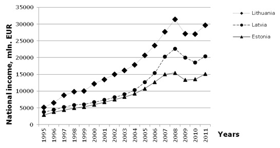 |
| Figure 1. The national income of the Baltic States over the period of 1995–2011 |
The data on the government debt for all Baltic countries were retrieved from Eurostat database (Eurostat, 2013). Figures on debt were taken in actual costs, too, in millions of EUR (Figure 2).
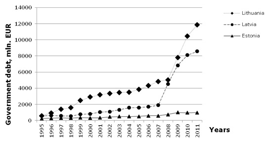 |
| Figure 2. The government debt of the Baltic States over the period of 1995–2011 |
2. Domar’s Models
The models, considered in the present article, are the Domar’s model of the constant national income growth rate, referred further in this paper as a “classic Domar’s model” and the “War” Domar’s model, referred further as a “war model”. In both models, the national income increases at a constant percentage rate r. In such a case, the national income Y at the year t is given by
 , , |
(1) |
where Y0 is the national income at the beginning of the period under consideration.
In the classic Domar’s model, the newly accumulated government debt is formed by a borrowing a percent of the national income each year. Thus, the total amount of debt, D, accumulated by the year t is:
 , , |
(2) |
where D0 is the “initial” government debt at the beginning of the period of interest. The main outcome of the classic Domar’s model is the conclusion that if the national income increases at the constant rate, the ratio of the debt to the national income in a long term run tends to finite constant:
 , , |
(3) |
The same is true for the tax burden, required to pay interests on the debt. Given i is the interest ratio, paid on the debt, the percent of the taxes to be collected to pay the interest U/T tends to
 , , |
(4) |
Here U = iD is an interest charge on the debt and T = Y+U is a taxable income. Thus the tax burden required to keep up with the debt is a limited value, too, entirely defined by the national income growth rate r, the percentage of the national income yearly borrowed by the government a and the interest rate on the debt i. Although limited, the tax burden may reach levels, intolerable for economy, at certain values of r, a and i, especially for i >> r. In his work, Domar considered the time period of 300 years, and the convergence of D/Y and U/T to the limit values was observed after approximately 150 years.
The Domar’s “war model” differs from the “classic” one by consideration of two alternating periods: the “peace” period, when the government borrows a low percent of the national income a, and the “war” period, when the borrowing ratio increases to a higher level b. In the war model, the national income still remains growing in accord with eq.1. Equation 2, in turn, has to be rewritten to be adapted to the two periods of different borrowing policies. For calculation, it is more convenient to rewrite both eq.1 and eq.2 in the form
 , , |
(5) |
 , , |
(6) |
where Yn-1 and Dn-1 is the national income and the government debt at the end of the previous period and an is the percentage of the national income, borrowed yearly in the current period, i.e. a in the peace period and b in the war period. The outcome of the Domar’s war model is similar to one of the classic model: both average ratio D/Y and the tax burden converge to the limited values, although yearly values of D/Y and U/T oscillate between limited minimal (in the peace period) and maximal (at “war”) values. In the original work, Domar analysed the 30-year period, divided into 25 years of peace and 5 years of war. In the present paper, a ten-year period is analysed.
3. Crisis Model
The assumption of the Domar’s model of constant growth rate of the national income seems unrealistic for the real economy, where the periods of growth are replaced with the periods of recession. Thus, for analysis of the situation in Baltic States in 1995–2011, author modifies the Domar’s model to account for the crisis. By analogy with the Domar’s war model, two periods are considered. In the “growth period”, the national income increases with the rate rA and the government borrows a percents of the national income each year. At the “recession period”, the national income increases with the rate rB (that may be negative), but the government borrows at a higher rate b to compensate the decrement of the national income. To match the model to the actual situation, the lag between the beginning of the crisis and the drop in the national income may be introduced. The model equations for the growth period are:
 , , |
(7) |
 , , |
(8) |
where Yn-1 and Dn-1 is the national income and the government debt at the end of the previous recession period. For the recession period, the form of the equation is one of the eqs.7, where rA is replaced with rB, a with b, and Yn-1 and Dn-1 is the national income and the government debt at the end of the previous growth period.
4. The Governmental Debt of the Baltic States in 1995–2011
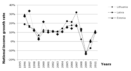
The analysis of the national income growth rate over the 16 year period (Figure 3) demonstrates that in all the Baltic States the national income growth ratio dropped two times, in 1998–1999 and in 2008–2010, with r reached the smallest value in 1999 and 2009 respectively. Such behaviour is in a good agreement with the economic cycle model, proposed by Juglar (Lee, 1955). The Juglar cycles appear with periodicity of 8–11 years with some fluctuations in the cycles’ duration. From the analysis of Figure 3 data, the 10-year period was used for calculation in the present paper. One has to note, that the crisis of 1998–1999 was attributed only by a slight drop in the national income growth rate. There was no drop in the national income itself, as well as no government borrowing. This may be explained by the low level of national income of the Baltic States, especially one of Latvia and Estonia at that time and the moderate severity of the crisis. Besides, in 2008–2009, the national income growth rate dropped to a negative value. One have to not, that during the period of 2000–2004 all Baltic countries demonstrated nearly the same growth of 10% that may be thought as “intrinsic” growth rate for developing Baltic economies.
|
| Figure 3. The national income growth rate in the Baltic States in 1995–2011 |
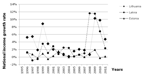
The borrowing policy of the Baltic States is illustrated by Figure 4. In 1999, Lithuania used the most intensive borrowing policy among all the Baltic countries, increasing borrowing rate up to 9% from the national income. This may be the reason of the peak rise of the Lithuanian national income growth rate in 2000. Latvia managed to cope with 1999 crisis without intensive borrowing, besides in 2008–2009 sharply raised borrowing rates up to nearly 12 %. Note, that Latvian government starts borrowing one year in advance to the maximal drop of the national income in 2009. Lithuania increased the borrowing rate in 2009 that coincides with the maximal drop in the growth rate. In contrast, Estonia kept the borrowing rate less than 2% all the time, in spite of the crisis.
The course of both the national income and the government debt growth in 1995–2011 was approximated, using the classic Domar’s model (eqs.1,2) , the Domar’s war model (eqs.5,6) and the proposed crisis model (eqs.7,8). The approximation was made by adjusting the models’ parameters (r, rA, rB, a, b) to minimize the root mean square deviation of the simulated values of the national income and the government debt from the actual ones. For instance, for the national income, it is calculated over n years as
 , ,
|
(9) |
|
| Figure 4. The borrowing ratios in the Baltic States in 1995–2011 |
|
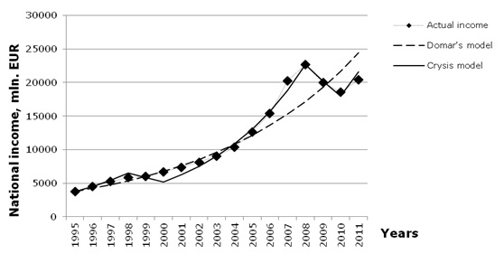
| Figure 5. National income growth for Latvia over the period of 1995–2011 |
For the crisis model, to approximate the national income growth, the period of 10 years was split into 8-year period of growth with positive rA and 2-year period of recession with negative rB. Such division takes into account a one-year lag between the beginning of the crisis and the observable decrease of the national income, so the crisis itself begins at the last year of the 8-year growth period. The result of the national income growth approximation for Latvia is demonstrated at the Figure 5. For the classic Domar’s model, the rate of national income growth r was equal to 11.7%, but s = 2247 mln EUR (for the Domar’s war model, the national income growth regularity was the same). For the crisis model, at the growth period rA = 18.5%, for recession rB = -11.7% and s is only 723 mln EUR. This means that the crisis model is more adequate for the description of the Latvian national income in the considered period. The same is true for other Baltic states: Table 1 demonstrates the crisis model provides a smaller approximation standard deviation for Lithuania and Estonia as well.
| Table 1 |
| Standard deviation for the Baltic States national income growth approximation over 1995–2011 (mln. EUR) |
|
“Classic” Domar’s model “War” Domar’s model |
Crisis model | |
| Latvia | 2274 | 723 |
| Lithuania | 3554 | 1393 |
| Estonia | 1749 | 764 |
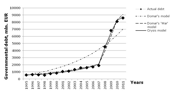
To approximate Latvian government debt growth in Domar’s war model and crisis model, the 10-years period was split into 7 years of “moderate” borrowing at rate a and 3 years of “extreme” borrowing at rate b. Such approach corresponds to the Latvian government policy to take into account the lag between the beginning of the crisis and the drop in national income, and to start intensive borrowing one year in advance, at the first signs of the crisis. Still, since the Latvian government didn’t borrow intensively during the 1998–1999 years crisis, for this period, the borrowing rate was assumed to be the same as in the growth period (i.e. when approximating the government debt growth, the crisis of 1998–1999 was not taken into account). The results of the Latvian government debt growth approximation are demonstrated in Figure 6.
|
| Figure 6. The government debt growth for Latvia over the period of 1995–2011 |
For Lithuania the period of “extreme” borrowing was shortened to 2 years, following data on the Figure 4, thus borrowing policy of Lithuania follows “8+2” pattern that corresponds to one of the national income itself. Moreover, for Lithuania, the borrowing during 1999 crisis have been taken into account, since borrowing rate at that time (9%) was close to one in 2009 (10%). For Estonia, Figure 4 does not demonstrate noticeable difference in borrowing rate during growth period and crisis period, so, for Estonia, the Latvian growth accumulation model was assumed for convenience of calculations. As it was in the case of national income approximation, the crisis model provides the best approximation of the government debt growth for both Latvia and Lithuania (Table 2). For Estonia, classic Domar’s model and crisis model performs equally well because of nearly constant borrowing rate over the all considered period.
Thus, one may conclude that the proposed crisis model provides the better approximation of the national income and the government debt growth in the Baltic States over the period from 1995 till 2011, thus only this model will be considered further. Table 3 summarizes parameters of the crisis model for Baltic countries.
| Table 2 |
| Standard deviation for the Baltic States government debt growth approximation over 1995–2011 (mln. EUR) |
| “Classic” Domar’s model | “War” Domar’s model | Crisis model | |
| Latvia | 1203 | 310 | 155 |
| Lithuania | 874 | 347 | 292 |
| Estonia | 53 | 63 | 52 |
One may note from the Table 3, that extremely high growth rate (18.5%) of the Latvian economics is attributed by highest drop in the income growth rate and most noticeable negative growth in recession period (-11.7%). Generally, all Baltic countries demonstrated steady growth at the rate of 10–13 % in 2001–2004. Such a high growth rate indicates that Baltic States still have a developing economy. It is unlikely that such a high rate will persist in the future, so one has to use more realistic data for the prognosis.
| Table 3 |
| The parameters of the national income and the government debt growth “crisis” model for Latvian economy in 1995–2011 |
| Latvia | Lithuania | Crisis model | |
| National income growth rate, % | |||
| “growth” period | 18.5 | 13.8 | 13.9 |
| “recession” period | -11.7 | - 5.9 | - 7.2 |
| Borrowing ratio, % | |||
| “growth” period | 0.9 | 1.4 | 0.3 |
| “recession” period | 12.9 | 9.3 | 0.8 |
Table 3 demonstrates the difference in the borrowing policy among Baltic Countries. For instance, Lithuania applies more active borrowing policy during “growth” period. Lithuanian borrowing ratio in this period (1.4%) is about 1.5 times higher then one of Latvia, and 5 times higher then one of Estonia. In contrary, during recession, the borrowing ratio for Lithuania (9.3%) remains nearly 25% less then one of Latvia (12.9%). Estonian borrowing ratio, being different in growth and recession period (0.3% and 0.8), is small.
5. Prognosis of the Governmental Debt in the Baltic States
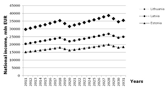
In this section, the short–term prognosis of the growth of the national income and government debt of the Baltic States is made on the basis of the considered “crisis” model. The prognosis, made up to year 2031, includes two full 10–year Juglar cycles. For the prognosis, the national income growth rate at the growth period was assumed to be equal to 2.5% for all Baltic States. This rate was taken from the prognosis made by the International Monetary Fund for European countries (IMF, 2012). For the crisis period, the national income drops at the rate of –5%. This “crisis” rate was obtained, assuming the drop of r from the growth period level to be equal to the one during the “moderate” 1998–1999 crisis (that assumed from Figure 3 to be equal to 7.5% for all Baltic countries). Under such assumptions, the dynamics of the national income growth is shown in Figure 7. Note, that even under the influence of the regular crisis, the national income still increases in general.
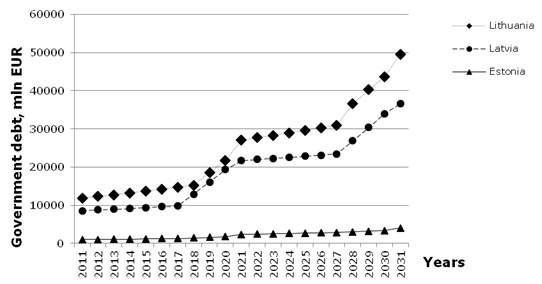
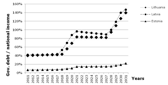
The accumulation of the government debt was predicted, using parameters a and b of the government borrowing policy, that was obtained from approximation of 1995–2011 years data and summarized in the Table 3. The predicted values of the government debt are shown at the Figure 8, but the ratio “government debt/ national income” – in Figure 9.
|
| Figure 7. Prognosis of the national income of the Baltic States |
|
| Figure 8. Prognosis of the government debt of the Baltic States |
Although in absolute figurers the governmental debt for Lithuania is the highest, the ratio “debt/income” is highest for Latvia. The difference in accumulation of government debt may appear due to different “borrowing pattern”: the lag between dept increment in Latvia and Lithuania is due to model assumption that Lithuania starts to borrow at the crisis peak. It worth to note, that the ratio “debt/income” increases over time for Estonia, too, despite of moderate borrowing policy. The proposed model does not show any traces of saturation in “debt / income” regularity in a short-term period. This is a difference from the Domar’s model: the latter demonstrated that in a long term run “debt / income” ratio tends to some finite value (Domar, 1944).
|
| Figure 9. Prognosis of the government debt to national income ratio for the Baltic States |
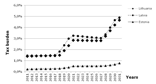
Figure 10 shows prognosis for the tax burden, required to pay off the interest on the government debt. The tax calculations were made, assuming the public debt interest to be equal to 3.5%, which is the actual interest, paid by Latvian government in 2011. The results show, that given the governments implement the same borrowing policy, as it was done in 2008–2010, the burden of debt will require about 5% of the national income to be paid as an interest in 2030-ies for both Latvia and Lithuania. For Estonia, the tax required to pay off interests on government debt remains within 1% from the national income.
|
| Figure 10. Prognosis of the tax burden to pay off interest on government debt |
The analysis of the “debt/income” curve and of the tax burden curves (Figure 9, 10) shows, that the fast burden growth takes place at the recession period, when the governments increase borrowing. In the growth periods, the tax burden tends to decrease, even when the interest rate on the debt is higher, then the rate of the national income growth.
Thus, one may conclude, that the government may use intensive borrowing time-to-time at the crisis, to cope with the drop in the national income, besides it should not become a regular practice, since the growth in the tax burden will be intolerable. In order to keep it under 2% within next 30 years, one have to recommend avoiding intensive 2008 – style borrowing during next crisis waves in 2018–2020 and 2028–2030.
Conclusions
- The proposed crisis model provides an adequate description of the accumulation of the government debt in the Baltic States in 1995–2011, better than the “war” model of Domar.
- In the short run, the crisis model predicts the tax burden grows up to nearly 5% in 30 years for Lithuania and Latvia, given the state borrowing policy doesn’t change in comparison with 2008–2010.
- To keep the tax burden low, the state has to forecast for the crisis to avoid intensive borrowing at the crisis time.
Bibliography
Arai, R. (2011). Productive Government Expenditure and Fiscal Sustainability. FinanzArchiv: Public Finance Analysis, Mohr Siebeck, Tübingen, Volume 67, Issue 4, December, pp. 327–351
Avramovic D (1964). Economic Growth and External Debt. Baltimore: The Johns Hopkins Press. xiii.
Central Statistical Bureau of Latvia (2012). Retrieved: http://www.csb.gov.lv/en/dati/key-indicators-30780.html. [Accessed: 05.11.2012.]
Domar, E. (1944). The “Burden of the Debt” and the National Income. The American Economic Review, Volume 34, Issue 4, pp. 798–827
Eurostat database (2013), Retrieved: http://epp.eurostat.ec.europa.eu. [Accessed: 05.02.2013.]
International Monetary Fund (2012). The World Economic Outlook, April 2012, Retrieved http://www.imf.org/external/pubs/ft/weo/2012/01/, [Accessed: 09.11.2012.]
Keunsuk, C.A., Stephen, J.T. (2010). Foreign Debt Supply in an Imperfect International Capital Market: Theory and Evidence. Journal of International Money and Finance, Elsevier, Volume 29, Issue 2, pp. 201–223
Lee, M.W. (1955). Economic Fluctuations. Homewood, IL: Richard D. Irwin.
Sardoni, C. (2008). The sustainability of fiscal policy: an old answer to an old question? Proc. of the conference “Macroeconomic Policies on Shaky Foundations – Whither Mainstream Economics?”, 31 October – 1 November 2008, Berlin, Retrieved: http://www.boeckler.de/pdf/v_2008_10_31_sardoni.pdf. [Accessed: 19.10.2012.]